
Online Course Notes: Udacity A/B Testing Final Project
1. Introduction
This is the final project of the online course Udacity A/B Testing by Google. It’s based on an actual experiment that was run by Udacity. The specific numbers have been changed, but the patterns have not. Let me walk you through about how to design the experiment, analyze the results, and propose a high-level follow-on experiment. The project instructions contain more details.
1.1 Experiment Overview
You can find the detailed overview in above instruction link, here let me introduce it briefly.
Current
At the time of this experiment, Udacity courses currently have two options on the course overview page: start free trial, and access course materials. If the student clicks start free trial, they will be asked to enter their credit card information, and then they will be enrolled in a free trial for the paid version of the course. After 14 days, they will automatically be charged unless they cancel first. If the student clicks access course materials, they will be able to view the videos and take the quizzes for free, but they will not receive coaching support or a verified certificate, and they will not submit their final project for feedback.
Changes that require A/B Testing
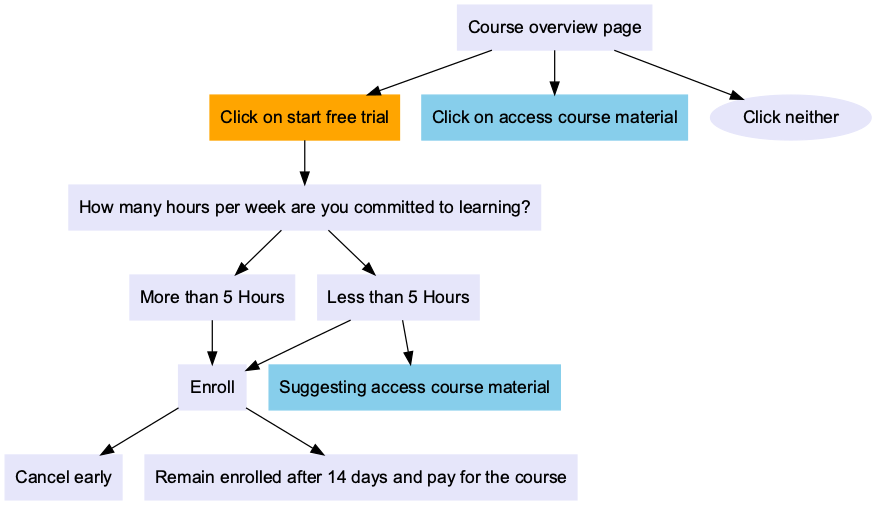
In the experiment, Udacity tested a change where if the student clicked start free trial, they saw a pop up modal that asked them how much time they had available to devote to the course. The critical value was 5 hours:
- If the student indicated 5 or more hours per week, they would be taken through the checkout process as usual.
- If they indicated fewer than 5 hours per week, a message would appear indicating that Udacity courses usually require a greater time commitment for successful completion, and suggesting that the student might like to access the course materials for free. At this point, the student would have the option to continue enrolling in the free trial, or access the course materials for free instead.
The screenshot below shows what the experiment looks like:

Here are the flow diagrams:
Hypothesis
The hypothesis was that this might set clearer expectations for students upfront, thus reducing the number of frustrated students who left the free trial because they didn’t have enough time—without significantly reducing the number of students to continue past the free trial and eventually complete the course. If this hypothesis held true, Udacity could improve the overall student experience and improve coaches’ capacity to support students who are likely to complete the course.
1.2 Datasets
Rough Estimates of the Baseline Values: This spreadsheet contains rough estimates of the baseline values, we are going to use it for pre-test analysis, in other words, we will design the A/B test based on its data.
Test Results: This spreadsheet contains the test results, we are going to analyze it to decide if the change has any effect.
3. Experiment Design
According to the instructions, the unit of diversion of this experiment is a cookie, although if the student enrolls in the free trial, they are tracked by user-id from that point forward. The same user-id cannot enroll in the free trial twice. For users that do not enroll, their user-id is not tracked in the experiment, even if they were signed in when they visited the course overview page.
Our next step is to /figsure out the Invariant Metrics and Evaluation Metrics. The following are the possible metrics:
- Number of cookies: That is, number of unique cookies to view the course overview page. (\(d_{min} = 3000\))
- Number of user-ids: That is, number of users who enroll in the free trial. (\(d_{min} = 50\))
- Number of clicks: That is, number of unique cookies to click the “Start free trial” button (which happens before the free trial screener is trigger). (\(d_{min} = 240\))
- Click-through-probability: That is, number of unique cookies to click the “Start free trial” button divided by number of unique cookies to view the course overview page. (\(d_{min} = 0.01\))
- Gross conversion: That is, number of user-ids to complete checkout and enroll in the free trial divided by number of unique cookies to click the “Start free trial” button. (\(d_{min} = 0.01\))
- Retention: That is, number of user-ids to remain enrolled past the 14-day boundary (and thus make at least one payment) divided by the number of user-ids to complete checkout. (\(d_{min} = 0.01\))
- Net conversion: That is, number of user-ids to remain enrolled past the 14-day boundary (and thus make at least one payment) divided by the number of unique cookies to click the “Start free trial” button. (\(d_{min} = 0.0075\))
3.1 Choosing Invariant Metrics
Invariant metrics shouldn’t change because of the experiment change, so we must select metrics that happen before the experiment change is trigger. In other words, the good invariant metrics are those happen before seeing the pop up modal.
Here is the table of those metrics and their baseline values:
| Invariant Metric | Formula | \(d_{min}\) | Baseline Value |
|---|---|---|---|
| Number of cookies | \(C_{cookies}\) = # of unique cookies to view the course overview page | 3000 | 40000 |
| Number of clicks | \(C_{clicks}\) = # of unique cookies to click the “Start free trial” button | 240 | 3200 |
| Click-through-probability | CTP = \(\displaystyle \frac{C_{clicks}}{C_{cookies}}\) | 0.01 | 0.08 |
3.2 Choosing Evaluation Metrics
In contrast to invariant metrics, evaluation metrics will be affected by the change of experiment and vary between control and treatment group.
Here is the table of those evaluation metrics and their baseline values:
| Metric | <p align="left">Formula</p> | dmin | Baseline Value |
|---|---|---|---|
| Gross Conversion | <p align="left">\(\displaystyle{GC = }\frac{C_{enrollments}}{C_{clicks}}\)</p> | 0.01 | 0.20625 |
| Retention | <p align="left">\(\displaystyle{R = }\frac{C_{payments}}{C_{enrollments}}\)</p> | 0.01 | 0.53 |
| Net Conversion | <p align="left">\(\displaystyle{NC = }\frac{C_{payments}}{C_{clicks}}\)</p> | 0.0075 | 0.1093125 |
Actually, \(\displaystyle \text{Retention} = \frac{\text{Net conversion}}{\text{Gross conversion}}\), so we probably don’t need all 3 metrics, knowing any 2 metrics can calculate the 3rd one. Let’s dig deeper and decide which one to be ignored.
3.3 Calculating Standard Error
Requirement
For each metric we selected as an evaluation metric, make an analytic estimate of its standard error, given a sample size of 5000 cookies visiting the course overview page. Enter each estimate in the appropriate box to 4 decimal places
Hint 1: Make sure use only the information given in the Rough Estimates of the Baseline Values. Do not use Test Results, since this step should be done before the experiment is run.
Hint 2: Make sure to find out how many units of analysis will correspond to 5000 pageviews for each metric. Again, use the given Rough Estimates of the Baseline Values.
Formula
The formula is
\[\displaystyle SE = \sqrt{\frac{p \cdot (1-p)}{n}}\]Where \(p\) is proportion of successes in the sample, \(n\) is the number of observations in the sample, both values can be found in Rough Estimates of the Baseline Values.
Read baseline values
import pandas as pd
import numpy as np
import math
from scipy.stats import norm

baseline = pd.read_csv("data/Udacity-AB-Testing-Final-Project-Baseline-Values.csv")
baseline
| Metric | Baseline Value | |
|---|---|---|
| 0 | Unique cookies to view course overview page pe... | 40000.000000 |
| 1 | Unique cookies to click "Start free trial" per... | 3200.000000 |
| 2 | Enrollments per day: | 660.000000 |
| 3 | Click-through-probability on "Start free trial": | 0.080000 |
| 4 | Probability of enrolling, given click: | 0.206250 |
| 5 | Probability of payment, given enroll: | 0.530000 |
| 6 | Probability of payment, given click | 0.109313 |
Our next step is to create functions to calculate standard errors, based on above baseline values.
# Baseline values of those metrics
cookies = 40000
clicks = 3200
enrollments = 660
CTP = 0.08
gross_conversion = 0.20625
retention = 0.53
net_conversion = 0.1093125

# Dictonary of Gross conversion
GC = {}
GC['p'] = gross_conversion
GC['d_min'] = 0.01
GC['n'] = clicks

# Dictonary of Retention
R = {}
R['p'] = retention
R['d_min'] = 0.01
R['n'] = enrollments

# Dictonary of Net Conversion
NC = {}
NC['p'] = net_conversion
NC['d_min'] = 0.0075
NC['n'] = clicks

# Create the function to calculate Standard Error
def calculate_se(p, n):
    SE = np.sqrt(p * (1-p) / n)
    return round(SE, 4)

GC['SE'] = calculate_se(GC['p'], GC['n'])
R['SE'] = calculate_se(R['p'], R['n'])
NC['SE'] = calculate_se(NC['p'], NC['n'])

evaluation_metrics = pd.DataFrame(
    {
        "Standard Error (n=40000)": [
            calculate_se(GC["p"], GC["n"]),
            calculate_se(R["p"], R["n"]),
            calculate_se(NC["p"], NC["n"])
        ]
    },
    index=["Gross conversion", "Retention", "Net conversion"]
)

evaluation_metrics
| Standard Error (n=40000) | |
|---|---|
| Gross conversion | 0.0072 |
| Retention | 0.0194 |
| Net conversion | 0.0055 |
Scaling
We’ve known the standard errors for 40000 cookies (see the spreadsheet of baseline values ). But the requirement is to get the standard error when n=5000 cookies, according to the formula, standard error is proportional to \(\displaystyle \sqrt{\frac{1}{n}}\), so the standard errors of n=5000 will be larger than n = 40000, with a ratio \(\displaystyle \sqrt{\frac{40000}{5000}}\).
evaluation_metrics['Standard Error (n=5000)'] = round(evaluation_metrics['Standard Error (n=40000)'] * np.sqrt(40000/5000), 4)

evaluation_metrics
| Standard Error (n=40000) | Standard Error (n=5000) | |
|---|---|---|
| Gross conversion | 0.0072 | 0.0204 |
| Retention | 0.0194 | 0.0549 |
| Net conversion | 0.0055 | 0.0156 |
3.4 Calculating Sample Size
In order to obtain meaningful results, we want our test to have sufficient statistical power (\(1- \beta\)). As sample size increases, the statistical power increases, but the trade-off is the probability of getting Type I error increases as sample size increases. Therefore, it’s important to choose appropriate sample size to get a balance.
In this project, \(\alpha = 0.05, \beta = 0.2\), they are the most common Type I error rate and Type II error rate (Reference Type I and Type II errors).
There are multiple methods to calculate the sample size, here we will try 2 of them.
Method 1: Formula
The formula for estimate minimum sample size of each group (two-sided test) is as follows:
\[\displaystyle N = \frac{(z_{1-\alpha/2} + z_{1-\beta})^2 \cdot (\sigma_{1}^2 + \sigma_{2}^2)}{\delta^2}\]where \(\sigma = \left\lvert{u_{2} - u_{1}}\right\rvert\), the means and variances of the two respective groups are (\(u_{1}, \sigma_{1}^2\)) and (\(u_{2}, \sigma_{2}^2\))
Above is the general formula, in the pre-analysis of A/B testing, we can use the following values:
- \[u_{1} = p_{baseline}\]
- \[u_{2} = p_{baseline} + d_{min}\]
- \[\delta = d_{min}\]
- \[\sigma_{1}^2 = p_{baseline} \cdot (1- p_{baseline})\]
- \[\sigma_{2}^2 = (p_{baseline} + d_{min}) \cdot (1- (p_{baseline} + d_{min}))\]
Let’s calculate the sample size by the following code.
def get_z_score(cd):
    # cd is the cumulative density
    return norm.ppf(cd)

def sample_size(p1, p2, alpha=0.05, beta=0.2):
    z1 = get_z_score(1 - alpha/2)
    z2 = get_z_score(1 - beta)
    d = p2 - p1
    z = z1 + z2
    v1 = p1 * (1-p1)
    v2 = p2 * (1-p2)
    v = v1 + v2
    n = z**2 * v / d**2

    return int(math.ceil(n))

# calculate sample sizes
GC['Sample Size'] = sample_size(p1=GC['p'], p2=GC['p']+GC['d_min'])
R['Sample Size'] = sample_size(p1=R['p'], p2=R['p']+R['d_min'])
NC['Sample Size'] = sample_size(p1=NC['p'], p2=NC['p']+NC['d_min'])

evaluation_metrics["Sample Size (Method 1)"] = [
    GC["Sample Size"],
    R["Sample Size"],
    NC["Sample Size"]
]

evaluation_metrics
| Standard Error (n=40000) | Standard Error (n=5000) | Sample Size (Method 1) | |
|---|---|---|---|
| Gross conversion | 0.0072 | 0.0204 | 26153 |
| Retention | 0.0194 | 0.0549 | 39049 |
| Net conversion | 0.0055 | 0.0156 | 27982 |
Method 2: Sample Size Calculator
One of the most common online calculator is Sample Size Calculator by Evan Miller.
For example, below is the screen shot of Gross conversion’s sample size:
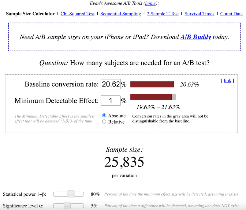
Similarly, we can get the sample sizes of the other 2 metrics, let’s manually add them to the evaluation_metrics dataframe.
evaluation_metrics["Sample Size (Method 2)"] = [25835, 39115, 27413]

evaluation_metrics
| Standard Error (n=40000) | Standard Error (n=5000) | Sample Size (Method 1) | Sample Size (Method 2) | |
|---|---|---|---|---|
| Gross conversion | 0.0072 | 0.0204 | 26153 | 25835 |
| Retention | 0.0194 | 0.0549 | 39049 | 39115 |
| Net conversion | 0.0055 | 0.0156 | 27982 | 27413 |
As we can see, the sample sizes of Method 1 and Method 2 are very close, which means our calculation is correct. In later analysis, let’s use the sample sizes of Method 2.
3.4.1 How Many Pageviews are Required?
Knowing the sample size is not the end, because the unit of the 3 metrics are different. Gross conversion and Net conversion are based on # of clicks, while Retention is based on # of enrollment, none of them is unit of the diversion, i.e., the cookie that viewing course overview page.
According to the baseline values, their relationships are:
- every 40000 cookies that view course overview page \(\Rightarrow\) 3200 clicks
so the ratio of gross conversion and net conversion is 40000/3200.
- every 40000 cookies that view course overview page \(\Rightarrow\) 660 enrollment
so the ratio of retention is 40000/660.
evaluation_metrics["Required pageviews (2 groups)"] = 2* evaluation_metrics["Sample Size (Method 2)"] * 40000/3200
evaluation_metrics.loc["Retention", "Required pageviews (2 groups)"] = 2* evaluation_metrics.loc["Retention", "Sample Size (Method 2)"] * 40000/660
evaluation_metrics["Required pageviews (2 groups)"] = evaluation_metrics["Required pageviews (2 groups)"].astype(int)
evaluation_metrics
| Standard Error (n=40000) | Standard Error (n=5000) | Sample Size (Method 1) | Sample Size (Method 2) | Required pageviews (2 groups) | |
|---|---|---|---|---|---|
| Gross conversion | 0.0072 | 0.0204 | 26153 | 25835 | 645875 |
| Retention | 0.0194 | 0.0549 | 39049 | 39115 | 4741212 |
| Net conversion | 0.0055 | 0.0156 | 27982 | 27413 | 685325 |
The maximum number of required pageview is 4741212, from Retention, it’s 7 times of the other 2 metrics, which means it will take 7 times longer to finish the test. As we’ve mentioned in 3.2 Choosing Evaluation Metrics, \(\displaystyle \text{Retention} = \frac{\text{Net conversion}}{\text{Gross conversion}}\), we can test the other 2 metrics instead.
So here we select 685325 as the required # of pageviews.
3.5 Choosing Duration and Exposure
We’ve known 685325 pageviews are required in this experiment. Our next step is to decide what fraction of Udacity’s traffic is divert to this experiment, and then calculate the length of the experiment.
Fraction of traffic exposed
It’s a new change that affects the functionality of the “start free trial” button, we shouldn’t expose all the users to this experiment. On the other hand, the baseline value of Click-through-probability is 0.08, which means 8% of users at most will be affected when the button is not working, seems not too terrible.
Here, let’s expose 80% of the population to this experiment.
Duration
fraction_exposed = 0.8
daily_baseline_pageviews = 40000
daily_pageviews = fraction_exposed * daily_baseline_pageviews
evaluation_metrics["Duration (days)"] = evaluation_metrics["Required pageviews (2 groups)"]/daily_pageviews
evaluation_metrics["Duration (days)"] = evaluation_metrics["Duration (days)"].apply(np.ceil).astype(int)
evaluation_metrics
| Standard Error (n=40000) | Standard Error (n=5000) | Sample Size (Method 1) | Sample Size (Method 2) | Required pageviews (2 groups) | Duration (days) | |
|---|---|---|---|---|---|---|
| Gross conversion | 0.0072 | 0.0204 | 26153 | 25835 | 645875 | 21 |
| Retention | 0.0194 | 0.0549 | 39049 | 39115 | 4741212 | 149 |
| Net conversion | 0.0055 | 0.0156 | 27982 | 27413 | 685325 | 22 |
As we can learn from above table, the experiment duration to measure Retention is as long as 149 days, so we can insist our decision to remove that metric from our list.
The other 2 metrics have very close duration, here we select the longer one, 22 days, as the final duration.
3.6 Summary of the Design
Now we’ve finished the design of the experiment, below is the summary:
- Evaluation Metrics: Gross conversion and Net conversion
- Required # of pageviews in total: 685325
- Length of the experiment: 22 days
4. Experiment Results
The data for you to analyze is Test Results. This data contains the raw information needed to compute the above metrics, broken down day by day. Note that there are two sheets within the spreadsheet - one for the experiment group, and one for the control group.
The meaning of each column is:
- Pageviews: Number of unique cookies to view the course overview page that day.
- Clicks: Number of unique cookies to click the course overview page that day.
- Enrollments: Number of user-ids to enroll in the free trial that day.
- Payments: Number of user-ids who who enrolled on that day to remain enrolled for 14 days and thus make a payment. (Note that the date for this column is the start date, that is, the date of enrollment, rather than the date of the payment. The payment happened 14 days later. Because of this, the enrollments and payments are tracked for 14 fewer days than the other columns.)
4.1 Sanity Checks
We need to do some sanity checks to make sure this experiment are designed properly. Let’s start by checking whether invariant metrics are equivalent between the two groups.
Requirement
For each metric that we choose as an invariant metric, compute a 95% confidence interval for the value we expect to observe. Enter the upper and lower bounds, and the observed value, all to 4 decimal places.
Formula
For Pageviews and Clicks, they have binomial distribution, as we’ve mentioned in 3.3 Calculating Standard Error, the formula of standard error is:
\[\displaystyle SE = \sqrt{\frac{p \cdot (1-p)}{n}}\]The formula of confidence interval:
\[\displaystyle CI = [p - Z_{1-\alpha/2} \cdot SE, p + Z_{1-\alpha/2} \cdot SE]\]where \(\alpha\) is the Type I error rate, it’s 0.05 when the confidence level is 95%. The null hypothesis is there is no difference between the two groups, so p is 0.5.
As for CTP, there are two probabilities and we need to know the difference between them is significant or not, here is the formula of the standard error of the difference:
\[\displaystyle SE_{p_{2} - p_{1}} = \sqrt{SE_{p_{1}}^2 + SE_{p_{2}}^2} = \sqrt{\frac{p_{1}\cdot (1-p_{1})}{n_{1}} + \frac{p_{2}\cdot (1-p_{2})}{n_{2}}}\]We can improve the estimate of SE, when we expect null hypothesis is true, \(p_{1} = p_{2}\), so we can use the pooled estimate probability instead. The modified formula is:
\[\displaystyle SE_{p_{2} - p_{1}} = \sqrt{p_{pooled}\cdot (1-p_{pooled})\cdot (\frac{1}{n_{1}} + \frac{1}{n_{2}})}\]Import test results
For ease of calculation, the results of the experiment and the control group have been combined into a single file Udacity-AB-Testing-Final-Project-Experiment-Results.csv, the suffixes _con and _exp represent the result groups of the control group and the experiment, respectively.
# read test results
results = pd.read_csv('data/Udacity-AB-Testing-Final-Project-Experiment-Results.csv')

results.head()
| date | pageviews_con | clicks_con | enrollments_con | payments_con | pageviews_exp | clicks_exp | enrollments_exp | payments_exp | |
|---|---|---|---|---|---|---|---|---|---|
| 0 | Sat, Oct 11 | 7723 | 687 | 134.0 | 70.0 | 7716 | 686 | 105.0 | 34.0 |
| 1 | Sun, Oct 12 | 9102 | 779 | 147.0 | 70.0 | 9288 | 785 | 116.0 | 91.0 |
| 2 | Mon, Oct 13 | 10511 | 909 | 167.0 | 95.0 | 10480 | 884 | 145.0 | 79.0 |
| 3 | Tue, Oct 14 | 9871 | 836 | 156.0 | 105.0 | 9867 | 827 | 138.0 | 92.0 |
| 4 | Wed, Oct 15 | 10014 | 837 | 163.0 | 64.0 | 9793 | 832 | 140.0 | 94.0 |
results.info()
<class 'pandas.core.frame.DataFrame'>
RangeIndex: 37 entries, 0 to 36
Data columns (total 9 columns):
 #   Column           Non-Null Count  Dtype
---  ------           --------------  -----
 0   date             37 non-null     object
 1   pageviews_con    37 non-null     int64
 2   clicks_con       37 non-null     int64
 3   enrollments_con  23 non-null     float64
 4   payments_con     23 non-null     float64
 5   pageviews_exp    37 non-null     int64
 6   clicks_exp       37 non-null     int64
 7   enrollments_exp  23 non-null     float64
 8   payments_exp     23 non-null     float64
dtypes: float64(4), int64(4), object(1)
memory usage: 2.7+ KB
Enrollments and Payments have missing values, they only have data from Oct 11 to Nov 2. We need to keep that in mind, in later’s analysis that related to Gross conversion or Net conversion, we need to make sure to use the data during that period.
Sanity Check of Pageviews and Clicks
# get z-score when alpha = 0.05
alpha = 0.05
z_score = get_z_score(1 - alpha/2)

# initialize Pageviews and Clicks, with each group's sum results
for group in ["con", "exp"]:
    cookie_count = results[f"pageviews_{group}"].sum()
    clicks_count = results[f"clicks_{group}"].sum()
    if group == "con":
        control_list = [cookie_count, clicks_count]
    else:
        experiment_list = [cookie_count, clicks_count]

pageview_click_results = pd.DataFrame(
    {
        "Control": control_list,
        "Experiment": experiment_list
    },
    index=["Pageviews", "Clicks"]
)

# get total value of 2 groups
pageview_click_results["Total"] = pageview_click_results["Control"] + pageview_click_results["Experiment"]

# get expected/observed probability
pageview_click_results.loc[["Pageviews", "Clicks"], "Control Probability Observed"] = pageview_click_results["Control"]/pageview_click_results["Total"]
pageview_click_results.loc[["Pageviews", "Clicks"], "Control Probability Expected"] = 0.5

# get standard error
se_pageviews_expected = calculate_se(0.5, pageview_click_results.loc["Pageviews", "Total"])
se_clicks_expected = calculate_se(0.5, pageview_click_results.loc["Clicks", "Total"])

# get lower bound and upper bound of confidence interval
pageview_click_results["Standard Error"] = [se_pageviews_expected, se_clicks_expected]
margin = pageview_click_results["Standard Error"] * z_score
pageview_click_results["CI Lower Bound"] = pageview_click_results["Control Probability Expected"] - margin
pageview_click_results["CI Upper Bound"] = pageview_click_results["Control Probability Expected"] + margin
pageview_click_results = round(pageview_click_results, 4)

# check if the metric has statistical significance
def has_statistical_significance(observed, lower_bound, upper_bound):
    if lower_bound <= observed <= upper_bound:
        return False
    else:
        return True

pageview_click_results["Statistical Significant"] = pageview_click_results.apply(
    lambda x: has_statistical_significance(
        x["Control Probability Observed"],
        x["CI Lower Bound"],
        x["CI Upper Bound"],
    ),
    axis=1,
)

# create function to highlight True or False
def highlight_boolean(x):
    if x is True:
        color = 'lightgreen'
    elif x is False:
        color = 'pink'
    else:
        color = 'none'
    return 'background-color: %s' % color


pageview_click_results.style.applymap(highlight_boolean)
| Control | Experiment | Total | Control Probability Observed | Control Probability Expected | Standard Error | CI Lower Bound | CI Upper Bound | Statistical Significant | |
|---|---|---|---|---|---|---|---|---|---|
| Pageviews | 345543 | 344660 | 690203 | 0.500600 | 0.500000 | 0.000600 | 0.498800 | 0.501200 | False |
| Clicks | 28378 | 28325 | 56703 | 0.500500 | 0.500000 | 0.002100 | 0.495900 | 0.504100 | False |
Sanity Check of CTP
# get standard error of the difference of CTP
def calculate_diff_se(p_pooled, n1, n2):
    SE = np.sqrt(p_pooled * (1-p_pooled) * (1/ n1 + 1/ n2))
    return round(SE, 4)

ctp_results = pd.DataFrame(
    {
        "Control": [pageview_click_results.loc["Clicks", "Control"]/pageview_click_results.loc["Pageviews", "Control"]],
        "Experiment": [pageview_click_results.loc["Clicks", "Experiment"]/pageview_click_results.loc["Pageviews", "Experiment"]],
        "Total": [pageview_click_results.loc["Clicks", "Total"]/pageview_click_results.loc["Pageviews", "Total"]]
    },
    index=["CTP"]
)
ctp_results["Diff Expected"] = 0
ctp_results["Diff Observed"] = ctp_results["Experiment"] - ctp_results["Control"]

# get standard error
ctp_results["Standard Error"] = calculate_diff_se(
    ctp_results["Total"],
    pageview_click_results.loc["Pageviews", "Control"],
    pageview_click_results.loc["Pageviews", "Experiment"],
)

# get confidence interval
margin = ctp_results["Standard Error"] * z_score
ctp_results["CI Lower Bound"] = ctp_results["Diff Expected"] - margin
ctp_results["CI Upper Bound"] = ctp_results["Diff Expected"] + margin

# check if the difference has statistical significance
ctp_results["Statistical Significant"] = ctp_results.apply(
    lambda x: has_statistical_significance(
        x["Diff Observed"],
        x["CI Lower Bound"],
        x["CI Upper Bound"],
    ),
    axis=1,
)
ctp_results = round(ctp_results, 5)
ctp_results.style.applymap(highlight_boolean)
| Control | Experiment | Total | Diff Expected | Diff Observed | Standard Error | CI Lower Bound | CI Upper Bound | Statistical Significant | |
|---|---|---|---|---|---|---|---|---|---|
| CTP | 0.082130 | 0.082180 | 0.082150 | 0 | 0.000060 | 0.000700 | -0.001370 | 0.001370 | False |
Summary
None of them is statistical significant, which means all sanity checks of invariant metrics passed! We are good to move to the next step.
4.2 Result Analysis
4.2.1 Effect Size Tests
In this section, we need to check whether the test results of evaluation metrics are statistically and practically significant or not.
Null Hypothesis: Control group and Experiment group have same probability.
Alternative Hypothesis: Control group and Experiment group have different probability.
Similar to the previous step, we will need to compute a 95% confidence interval around the difference. As we’ve mentioned in 3.6 Summary of the Design, the evaluation metrics are Gross conversion and Net conversion. The formulas:
- \[\displaystyle {\text{Gross conversion(GC)} = }\frac{C_{enrollments}}{C_{clicks}}\]
- \[\displaystyle{\text{Net conversion(NC)} = }\frac{C_{payments}}{C_{clicks}}\]
- \[\displaystyle SE_{p_{2} - p_{1}} = \sqrt{p_{pooled}\cdot (1-p_{pooled})\cdot (\frac{1}{n_{1}} + \frac{1}{n_{2}})}\]
And don’t forget enrollments and payments have valid data during Oct 11 - Nov 2(the first 23 days) only.
# data from test results
sum_results = results.iloc[:23, :].sum()
control_clicks = sum_results.at['clicks_con']
experiment_clicks = sum_results.at['clicks_exp']
total_clicks = control_clicks + experiment_clicks
total_enrollments = sum_results.at['enrollments_con'] + sum_results.at['enrollments_exp']
total_payments = sum_results.at['payments_con'] + sum_results.at['payments_exp']

# create a dataframe of the 2 metrics
conversion_results = pd.DataFrame(
    {
        "Control": [sum_results.at['enrollments_con']/control_clicks,
                    sum_results.at['payments_con']/control_clicks],
        "Experiment": [sum_results.at['enrollments_exp']/experiment_clicks,
                    sum_results.at['payments_exp']/experiment_clicks],
        "Total": [total_enrollments/total_clicks,
                  total_payments/total_clicks],
    },
    index=["Gross conversion", "Net conversion"]
)

# get dmin from section "Designing the Experiment"
conversion_results["dmin"] = [0.01, 0.0075]

# check if the metric has practical significance, in this project, experiment group
# value is the observed value, control group value is the expected value (null hypothesis)
def has_practical_significance(observed, expected, dmin):
    if abs(observed-expected) >= dmin:
        return True
    else:
        return False


# calculate standard error, SE = np.sqrt(p_pooled * (1-p_pooled) * (1/ n1 + 1/ n2))
conversion_results["SE"] = np.sqrt(conversion_results["Total"]*(1-conversion_results["Total"])*(1/control_clicks+1/experiment_clicks))
margin = conversion_results["SE"] * z_score
conversion_results["CI Lower Bound"] = conversion_results["Control"] - margin
conversion_results["CI Upper Bound"] = conversion_results["Control"] + margin

# statistical significance
conversion_results["Statistical Significant"] = conversion_results.apply(
    lambda x: has_statistical_significance(
        x["Experiment"],
        x["CI Lower Bound"],
        x["CI Upper Bound"]
    ),
    axis=1
)

# practical significance
conversion_results["Practical Significant"] = conversion_results.apply(
    lambda x: has_practical_significance(
        x["Experiment"],
        x["Control"],
        x["dmin"]
    ),
    axis=1
)

conversion_results.style.applymap(highlight_boolean)
| Control | Experiment | Total | dmin | SE | CI Lower Bound | CI Upper Bound | Statistical Significant | Practical Significant | |
|---|---|---|---|---|---|---|---|---|---|
| Gross conversion | 0.218875 | 0.198320 | 0.208607 | 0.010000 | 0.004372 | 0.210306 | 0.227443 | True | True |
| Net conversion | 0.117562 | 0.112688 | 0.115127 | 0.007500 | 0.003434 | 0.110831 | 0.124293 | False | False |
We can learn from above table that Gross conversion is different between the 2 groups, experiment group has significant lower Gross conversion than control group. But Net conversion has no difference.
Next, let’s try another test and see if we will get the same results.
4.2.2 Sign Tests
The sign test is a statistical method to check whether the signs of the difference of the metrics between the experiment and control groups agree with the confidence interval of the difference. When the value of experiment group is larger than that of control group, the sign is positive, otherwise it’s negative.
Requirement
Run sign tests on Gross conversion and Net conversion, using the day-by-day data. For each metric, caculate its p-value, and indicate whether each result is statistically significant.
Get signs
First of all, we need to get the day-by-day sign.
# Get the first 23 days of data since it has no missing values
sign_test_data = results.iloc[:23, :].copy()
sign_test_data.set_index("date", inplace=True)

# The sign is "+1"/"-1" when experiment group value is larger/smaller than control group
sign_test_data["Control GC"] = sign_test_data["enrollments_con"]/sign_test_data["clicks_con"]
sign_test_data["Experiment GC"] = sign_test_data["enrollments_exp"]/sign_test_data["clicks_exp"]
sign_test_data["Control NC"] = sign_test_data["payments_con"]/sign_test_data["clicks_con"]
sign_test_data["Experiment NC"] = sign_test_data["payments_exp"]/sign_test_data["clicks_exp"]
sign_test_data["GC Sign"] = np.sign(sign_test_data["Experiment GC"] - sign_test_data["Control GC"]).astype(int)
sign_test_data["NC Sign"] = np.sign(sign_test_data["Experiment NC"] - sign_test_data["Control NC"]).astype(int)

sign_test_data = sign_test_data.loc[:, "Control GC":"NC Sign"]

# highlight signs
sign_test_data.style.applymap(lambda x: f"background-color: {'lightgreen' if x==1 else 'pink' if x==-1 else 'none'}")
| Control GC | Experiment GC | Control NC | Experiment NC | GC Sign | NC Sign | |
|---|---|---|---|---|---|---|
| date | ||||||
| Sat, Oct 11 | 0.195051 | 0.153061 | 0.101892 | 0.049563 | -1 | -1 |
| Sun, Oct 12 | 0.188703 | 0.147771 | 0.089859 | 0.115924 | -1 | 1 |
| Mon, Oct 13 | 0.183718 | 0.164027 | 0.104510 | 0.089367 | -1 | -1 |
| Tue, Oct 14 | 0.186603 | 0.166868 | 0.125598 | 0.111245 | -1 | -1 |
| Wed, Oct 15 | 0.194743 | 0.168269 | 0.076464 | 0.112981 | -1 | 1 |
| Thu, Oct 16 | 0.167679 | 0.163706 | 0.099635 | 0.077411 | -1 | -1 |
| Fri, Oct 17 | 0.195187 | 0.162821 | 0.101604 | 0.056410 | -1 | -1 |
| Sat, Oct 18 | 0.174051 | 0.144172 | 0.110759 | 0.095092 | -1 | -1 |
| Sun, Oct 19 | 0.189580 | 0.172166 | 0.086831 | 0.110473 | -1 | 1 |
| Mon, Oct 20 | 0.191638 | 0.177907 | 0.112660 | 0.113953 | -1 | 1 |
| Tue, Oct 21 | 0.226067 | 0.165509 | 0.121107 | 0.082176 | -1 | -1 |
| Wed, Oct 22 | 0.193317 | 0.159800 | 0.109785 | 0.087391 | -1 | -1 |
| Thu, Oct 23 | 0.190977 | 0.190031 | 0.084211 | 0.105919 | -1 | 1 |
| Fri, Oct 24 | 0.326895 | 0.278336 | 0.181278 | 0.134864 | -1 | -1 |
| Sat, Oct 25 | 0.254703 | 0.189836 | 0.185239 | 0.121076 | -1 | -1 |
| Sun, Oct 26 | 0.227401 | 0.220779 | 0.146893 | 0.145743 | -1 | -1 |
| Mon, Oct 27 | 0.306983 | 0.276265 | 0.163373 | 0.154345 | -1 | -1 |
| Tue, Oct 28 | 0.209239 | 0.220109 | 0.123641 | 0.163043 | 1 | 1 |
| Wed, Oct 29 | 0.265223 | 0.276479 | 0.116373 | 0.132050 | 1 | 1 |
| Thu, Oct 30 | 0.227520 | 0.284341 | 0.102180 | 0.092033 | 1 | -1 |
| Fri, Oct 31 | 0.246459 | 0.252078 | 0.143059 | 0.170360 | 1 | 1 |
| Sat, Nov 1 | 0.229075 | 0.204317 | 0.136564 | 0.143885 | -1 | 1 |
| Sun, Nov 2 | 0.297258 | 0.251381 | 0.096681 | 0.142265 | -1 | 1 |
For Gross conversion, there are 4 positive signs in 23 day-by-day tests. As for Net conversion, the number of positive signs is 10.
Then we can use Sign Test Calculator to get the p-value. Here is the screenshot of Gross conversion:
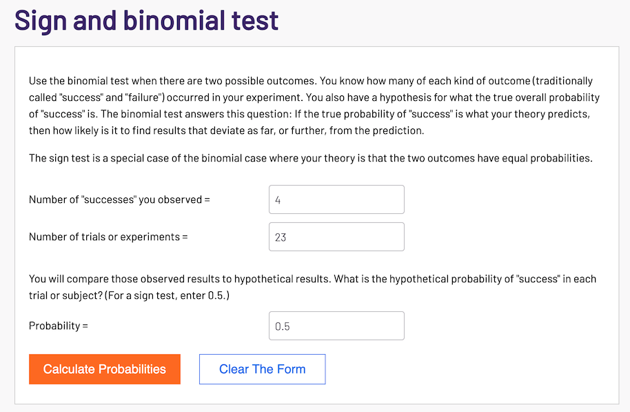
Sign Test Result
-
Gross conversion: p-value 0.0026 is less than 0.05, so it’s statistical significant.
-
Net conversion: p-value 0.6776 is larger than 0.05, so it’s not statistical significant.
In summary, the results of sign tests and effect size tests match.
4.3 Summary
The result of Gross conversion is significant, but Net conversion is not. In other words, after applying the change, enrollments has decreased but payments has no significant change.
5. Recommendations
Seems both the effect size tests and sign tests indicate the initial hypothesis is correct, that is, the Free Trial Screener could set clearer expectations for students up front, people who spent less than 5 hours per week probably didn’t enroll for free trial, that’s why Gross conversion decreased. Meanwhile, Net conversion has no significant change means the Free Trial Screener doesn’t significantly reduce the number of students that pay for it after the free trial.
However, there are some potential issues:
-
What if the decrease in Gross conversion is because some students don’t like the Free Trial Screener? After all, it takes extra steps to finish the enrollment with it.
-
Even though Net conversion has no significant change, but it just indicates students pay after 14 days’ free trial. We don’t know the number of students who complete the course will be increased or decreased.
-
Can this change really improve the student experience? Right now we don’t see any direct benefits from the test results.
Consequently, I would not recommend launching this Free Trial Screener feature for now. We need to understand the reason behind the decrease in Gross conversion, and we need concrete evidence shows the change is beneficial to Udacity, like improving the student experience or increasing revenue. Let’s talk with other team members and the manager about our concerns.
6. Follow-Up Experiment: Adding Detailed Introductions of Instructors
Requirement
Give a high-level description of the follow up experiment you would run, what your hypothesis would be, what metrics you would want to measure, what your unit of diversion would be, and your reasoning for these choices.
Overview of the Design
In this follow-up experiment, I would like to add a detailed introduction page for each instructor, and check if it can increase the click-through-probability on “Enroll now” button, that is, number of unique cookies to click the “Enroll now” button divided by number of unique cookies to view the course overview page. Here is the screeshot of course overview page with “Enroll now” button:

Note: After clicking “Enroll now” button, students need to enter the payment information. There is a 30 day free trial, after that, students will be charged automatically.
Current
Currently, each instructor’s introduction on the Udacity course overview page is short and very general. Therefore, users do not know how experienced those instructors are in this field, which makes the course less attractive.
Changes that require A/B testing
Create a detailed introduction page for each instructor, with more details like:
- What is the instructor’s field of expertise?
- How many years has the instructor been working in this field?
- The list of courses he/she instructs
- User ratings of those courses
And add a clickable link on the course overview page that can redirect users to that page. Here is the mock-up of course overview page:

The mockup of instructor’s introduction page:

Hypothesis
The hypothesis is by adding detailed introduction pages of instructors, user will find those instructors more professional and find the course more credible. Therefore, it can increase the Click-through-probability of “Enroll now” button.
Unit of Diversion
Cookies
Metrics
Invariant Metrics
Invariant metrics are those happen before the experiment change is trigger.
- Number of cookies: That is, number of unique cookies to view the course overview page. (\(d_{min}=3000\))
Evaluation Metrics
Evaluation metrics of this follow-up experiment are very similar to those of Free Trial Screener experiment. Some additional evaluation metrics have been added because the number of clicks may change.
- Number of clicks: That is, number of unique cookies to click the “Enroll now” button. (\(d_{min}=240\))
- Click-through-probability: That is, number of unique cookies to click the “Enroll now” button divided by number of unique cookies to view the course overview page. (\(d_{min}=0.01\))
- Number of user-ids: That is, number of users who complete the checkout and enrollment process. (\(d_{min}=50\))
- Gross conversion: That is, number of user-ids to complete the checkout and enrollment, divided by number of unique cookies to click the “Enroll now” button. (\(d_min=0.01\))
- Retention: That is, number of user-ids to remain enrolled past the 30-day boundary (and thus make at least one payment) divided by the number of user-ids to complete checkout. (\(d_{min}=0.01\))
- Net conversion: That is, number of user-ids to remain enrolled past the 30-day boundary (and thus make at least one payment) divided by the number of unique cookies to click the “Enroll now” button. (\(d_{min}=0.0075\))